From GPT-2 to Kimi Delta Attention: How Transformers Evolved into Modern AI Memory Systems
Twenty-two thousand five hundred and eighty. That is roughly how many GPT-2-scale models (≈124M parameters) fit inside Kimi K3 (≈2.8T parameters, 2026). Scale mattered—but it is not the whole story.
A parallel evolution happened inside the architecture itself:
AI models gradually changed from systems that repeatedly search every previous token into systems that maintain, update, erase, and selectively retrieve structured internal memories.
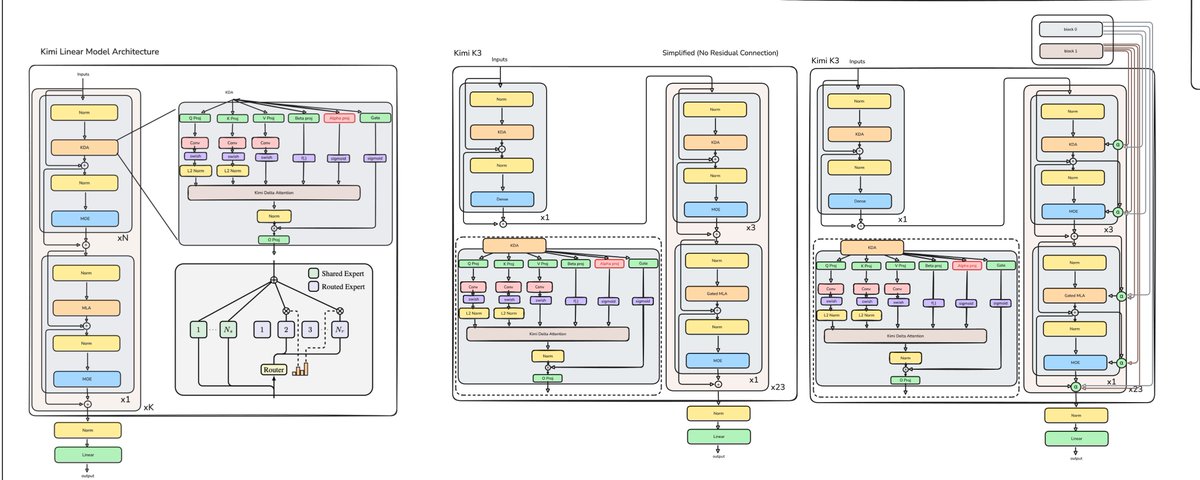
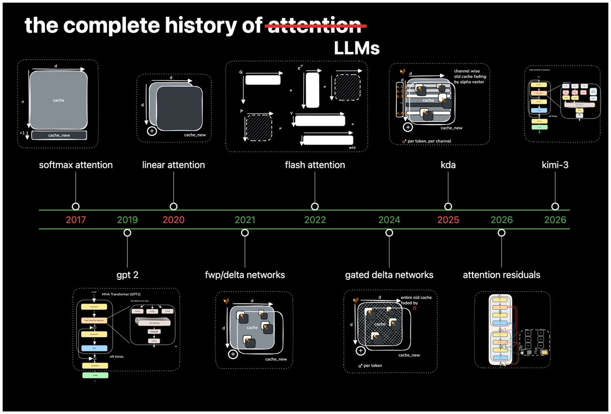
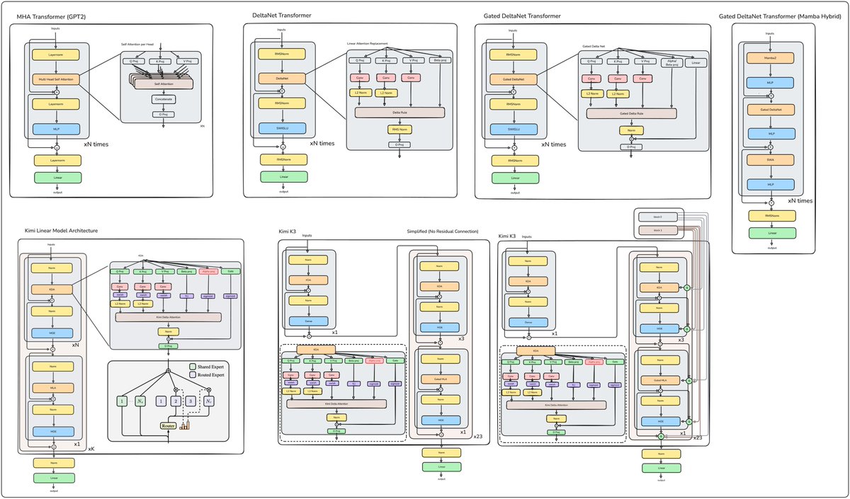
This article combines that memory-systems interpretation with the concrete architectural worklog 22580: From GPT2 to Kimi3, Explained by ali (@waterloo_intern), including the original diagrams, plus the research path from full softmax attention → linear attention → DeltaNet → Gated DeltaNet → Kimi Delta Attention → Kimi Linear / Kimi K3.
Introduction: scale and memory
The rise of modern AI is often told as larger models, more data, and more compute. That is only part of the story.
Inside the architecture, the progression is:
Full softmax attention
  → Linear attention
  → DeltaNet
  → Gated DeltaNet
  → Kimi Delta Attention (KDA)
  → Kimi Linear / Kimi K3 hybrid
| Generation | Main problem addressed |
|---|---|
| GPT-2-style full attention | Learning flexible global relationships between tokens |
| Linear attention | Quadratic attention cost and growing inference memory |
| DeltaNet | Interference when many key–value associations share compressed memory |
| Gated DeltaNet | Old information remaining in memory indefinitely |
| Kimi Delta Attention | Forgetting being too coarse-grained |
| Kimi Linear hybrid | Pure linear memory struggling with exact global retrieval |
| Kimi K3 | Depth dilution + sparse expert scale at trillion-parameter class |
This is not a simple replacement chain. Full attention remains extremely powerful because it provides direct access to individual tokens. Linear architectures gain efficiency by compressing history into a finite state—and compression introduces information loss.
Kimi Linear’s solution is therefore not to abandon full attention. It combines efficient KDA layers with periodic global attention (MLA) layers.
Attention is evolving from an expensive lookup mechanism into a learned memory-management system.
1. Before Transformers: sequential memory
Before the Transformer, language models were primarily recurrent:
- vanilla RNNs
- Long Short-Term Memory (LSTM)
- Gated Recurrent Units (GRU)
An RNN processes a sequence one token at a time:
The entire history must be compressed into one recurrent state. That created two major problems:
- Training was sequential — you could not compute token 100 before tokens 1–99.
- Long-range information degraded as it travelled through many recurrent updates.
The Transformer changed this by letting each token interact directly with other tokens.
2. The original Transformer: memory through attention
The 2017 Transformer removed recurrence from the main sequence-processing path and replaced it with self-attention (Attention Is All You Need). For every token representation x_t:
- query — what the current token is looking for
- key — what a token advertises
- value — what is returned when that token is selected
Simple example
“The customer submitted the application because she needed the loan.”
When processing “she,” the model can compare its query against keys for customer, application, loan, submitted, needed. The key for “customer” may win—so “she” incorporates that entity without routing information through every intermediate word.
Multi-head attention
Different heads can specialise (syntax, entity identity, temporal order, reference resolution, code dependencies). Head outputs are concatenated and projected again. This gave Transformers a flexible, content-addressable memory.
3. GPT-2: decoder-only general language model
GPT-2 showed that a large decoder-only Transformer trained on diverse web text could perform many tasks without a separate model per task (OpenAI technical report).
Largest published GPT-2 (approximate):
| Property | Value |
|---|---|
| Parameters | ~1.542B (largest); educational baseline often ~124M |
| Layers | 48 (large) / 12 (small) |
| Model dim | 1600 (large) / 768 (small) |
| Context | 1,024 tokens |
| Vocab | byte-level BPE ≈ 50,257 |
Autoregressive factorisation and causal attention
Position t may attend only to 1..t, never to the future. That decoder-only pattern became the foundation of many LLMs.
GPT-2 as code (conceptual)
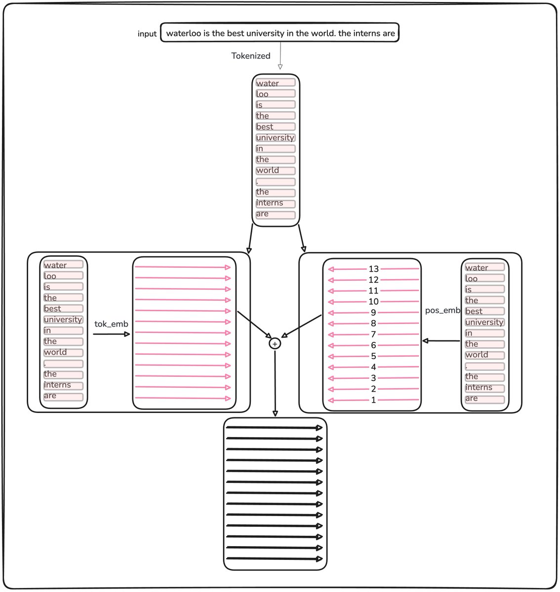
Token + position embeddings enter a stack of blocks; each block is pre-norm attention + MLP with residuals:
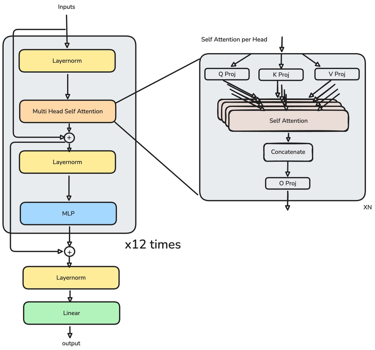
# Conceptual GPT-2 forward (decoder-only)
tok_emb = self.transformer.wte(idx)   # (b, t, n_embd)
pos_emb = self.transformer.wpe(pos)   # (t, n_embd)
x = self.transformer.drop(tok_emb + pos_emb)
for block in self.transformer.h:
    x = block(x)
x = self.transformer.ln_f(x)
logits = self.lm_head(x)
Causal attention (manual form):
q, k, v = self.c_attn(x).split(self.n_embd, dim=2)
# reshape to (B, n_head, T, head_dim)
att = (q @ k.transpose(-2, -1)) * (1.0 / math.sqrt(k.size(-1)))
att = att.masked_fill(causal_mask == 0, float("-inf"))
att = F.softmax(att, dim=-1)
y = att @ v
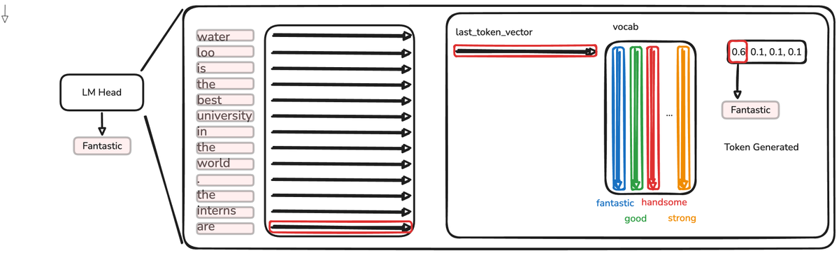
Without a KV cache, decoder-only generation recomputes representations for every prior position on each new token—even though only the final logits are consumed for the next-token choice.
Small GPT-2-style config (~124M):
vocab_size: int = 50304  # 50257 padded to multiple of 64
n_layer: int = 12
n_head: int = 12
n_embd: int = 768
At ~2.8T parameters, one Kimi K3 contains on the order of 22,580 such GPT-2-scale models—hence the worklog title.
4. What full attention does exceptionally well
Full softmax attention effectively retains an explicit list of previous keys and values. At generation time the model can ask: which previous token is most relevant to the current query?
Strengths:
- Direct retrieval — no need for facts to survive repeated recurrent compression.
- Dynamic relationships — the same token (“Python”) can mean language, animal, package, or repo depending on the query.
- High-capacity contextual memory — each earlier token keeps its own key/value.
That is why full attention remains strong for exact copying, code retrieval, multi-document reasoning, needle-in-a-haystack tests, and tracking many independent entities.
5. The quadratic attention problem
For context length n, pairwise query–key comparisons scale as O(n^2).
n = 1{,}000→ ~1M pairs per head (before layers/batches)n = 100{,}000→ ~10B pairs per head
Training: quadratic arithmetic in sequence length (FlashAttention reduces memory traffic; it does not remove pairwise work).
Inference: autoregressive decode stores prior keys/values in a KV cache. Per new token:
- compute grows with context length
- cache grows linearly with context
- memory bandwidth becomes a bottleneck
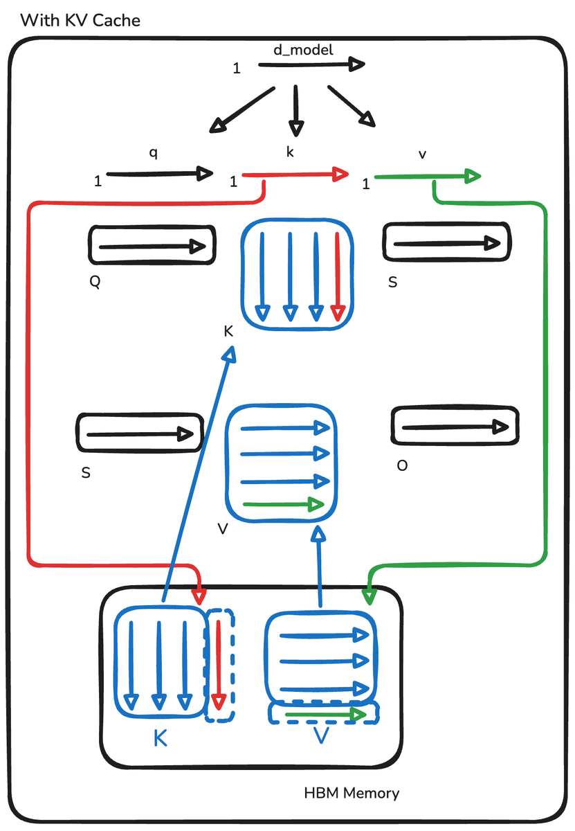
Modern workloads need far beyond GPT-2’s 1,024 tokens: repositories, tool traces, multi-hour chats, legal corpora, million-token agent trajectories. That demand pushed research toward linear sequence mechanisms.
6. Scaling transformed language models into modern AI
Architectural efficiency was only one track. In parallel:
- Scaling laws — loss often improved predictably with model size, data, and compute (Kaplan et al.).
- GPT-3 / in-context learning — the context became a temporary programming interface (instructions, demos, docs, tools) (Brown et al.).
- Instruction tuning / RLHF — aligning behaviour with human intent (InstructGPT).
- Sparse MoE — more total parameters without activating all of them every token (Switch Transformer).
The more models were used for in-context learning, retrieval, and agents, the more attention efficiency mattered.
7. Linear attention: compressed state instead of token archive
Linear attention reorganises the calculation so the model need not materialise a full n \times n matrix. Replace similarity with a feature map \phi:
Then multiplication can be reassociated as Q(K^\top V) rather than (QK^\top)V. A normalised recurrent form:
with updates S_t=S_{t-1}+\phi(k_t)v_t^\top, z_t=z_{t-1}+\phi(k_t).
This is linear in sequence length and reveals that a linear Transformer can also be a recurrent model with fixed-size state (Transformers are RNNs / linear attention).
Conceptual decode with ELU+1 feature map:
k = F.elu(k) + 1
q = F.elu(q) + 1
S, z = cache if cache is not None else (0.0, 0.0)
S = S + k.transpose(-1, -2) @ v   # accumulate associative memory
z = z + k.sum(...)                # normalisation state (sketch)
o = (q @ S) / (q @ z)
cache = (S, z)
Trade-off: the feature map is a less expressive approximation of the softmax kernel. Fidelity loss depends on architecture and workload—but the efficiency win is structural.
8. Why linear attention is revolutionary
| Full attention memory | Linear attention memory |
|---|---|
Archive {(k_i,v_i)} | Compressed matrix S_t |
Benefits:
- Constant recurrent memory (size depends on head dims, not
n) - Linear sequence processing
- Efficient autoregressive decoding (update fixed state vs scan growing KV)
- Streaming-friendly (unbounded stream without retaining every token)
Compression creates a new problem: interference.
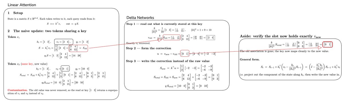
9. The interference problem
Additive update:
If the model writes k_A \rightarrow v_1 then later k_A \rightarrow v_2, a query with k_A may return a mixture. Similar keys also collide in overlapping regions of S.
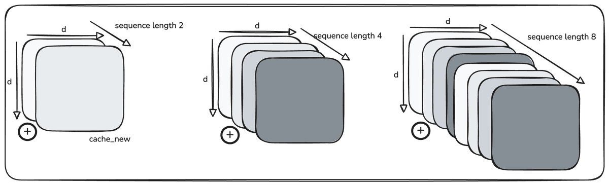
Whiteboard analogy: basic linear attention says “add the new note wherever space looks relevant” without first erasing conflicting content. Over time notes overlap and the board becomes unreadable.
Linear attention solved token-archive cost; it created the problem of controlling compressed memory. DeltaNet addressed that.
10. DeltaNet: correct memory before writing
DeltaNet applies the classical delta rule. First ask what the memory already predicts for the current key:
Framed as online gradient descent on reconstruction loss \tfrac{1}{2}\|S^\top k_t - v_t\|^2.
| Basic linear | DeltaNet |
|---|---|
S_t=S_{t-1}+k_tv_t^\top | write only the correction v_t - S_{t-1}^\top k_t |
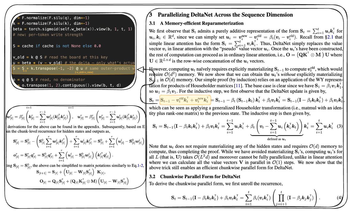
Conceptual PyTorch sketch:
q = F.normalize(F.silu(q), dim=-1)
k = F.normalize(F.silu(k), dim=-1)
beta = torch.sigmoid(self.w_beta(x))  # write strength
S = cache if cache is not None else 0.0
v_old = torch.einsum("...kd,...dv->...kv", k, S)  # read
u = beta * (v - v_old)                              # delta
S = S + torch.einsum("...kd,...kv->...dv", k, u)    # write
o = torch.einsum("...qd,...dv->...qv", q, S)
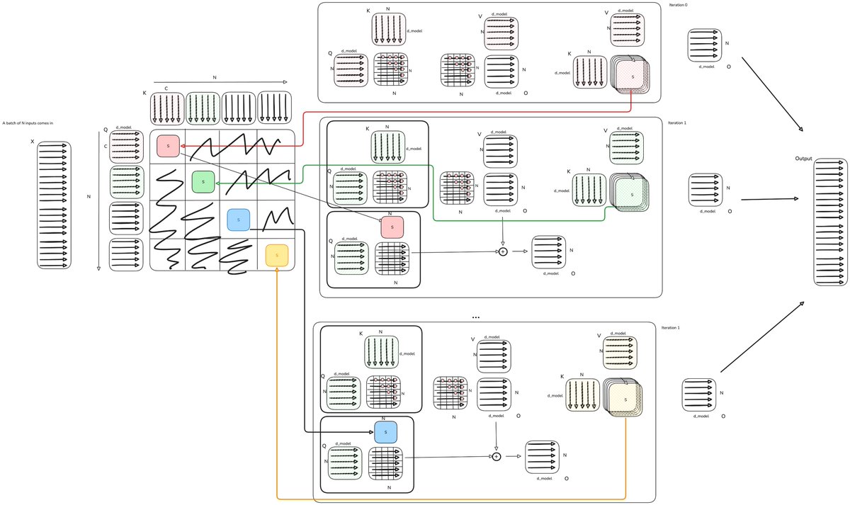
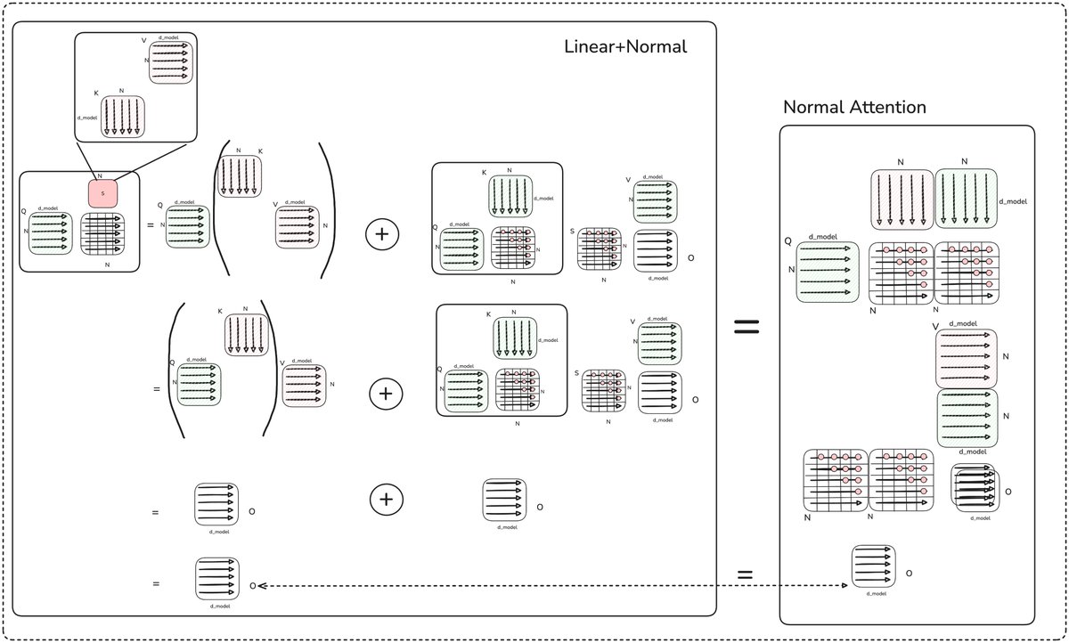
The 2024 DeltaNet work developed a hardware-efficient parallel algorithm over products of rank-one transforms, enabling scaled language modelling (e.g. 1.3B on 100B tokens with gains on recall-oriented tasks) (Parallelizing Linear Transformers with the Delta Rule).
Still missing: broad forgetting of stale, unqueried memory.
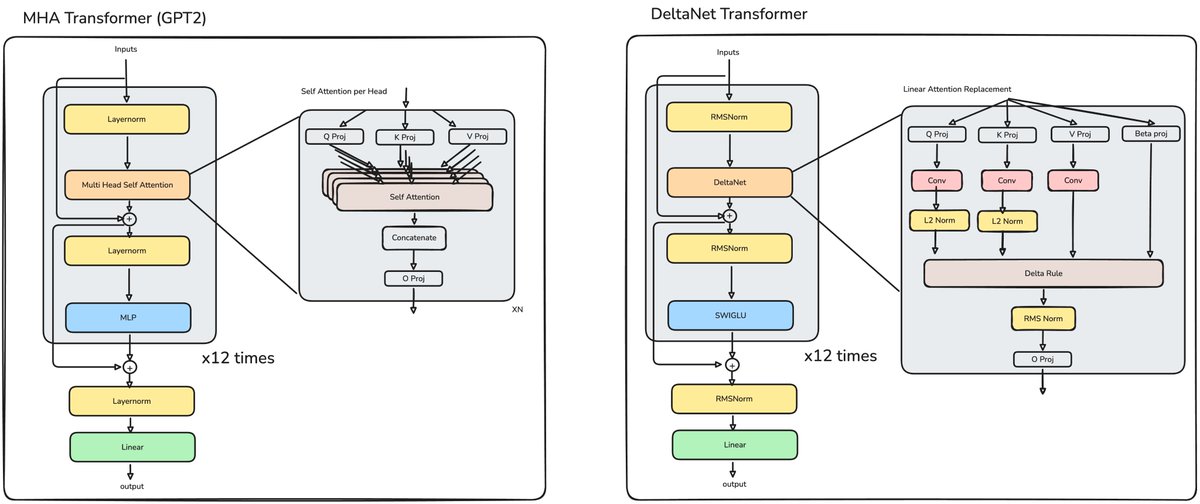
11. DeltaNet’s limitation: correction ≠ forgetting
DeltaNet can edit the mapping for the current key. It does not broadly forget information that is irrelevant, topic-shifted, or stale but not contradicted.
Example: mortgage discussion → unrelated insurance claim. Mortgage state may linger and consume finite capacity.
Difference:
- editing a memory vs
- managing its lifespan
12. Gated DeltaNet: correction + adaptive forgetting
Gated DeltaNet combines the delta rule with a learnable decay gate \alpha_t \in [0,1]:
\beta_t— how strongly to write/correct the current association\alpha_t— how much of the existing memory survives
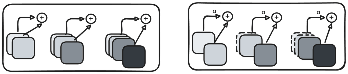
Pure additive linear attention could forget with cache = alpha * S_old + S_new. Uniform decay (as in Mamba-2 style gating) works but treats all associations equally. The delta rule can update one fact but cannot decay the rest. Gated DeltaNet combines both (Gated Delta Networks).
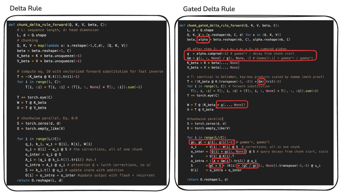
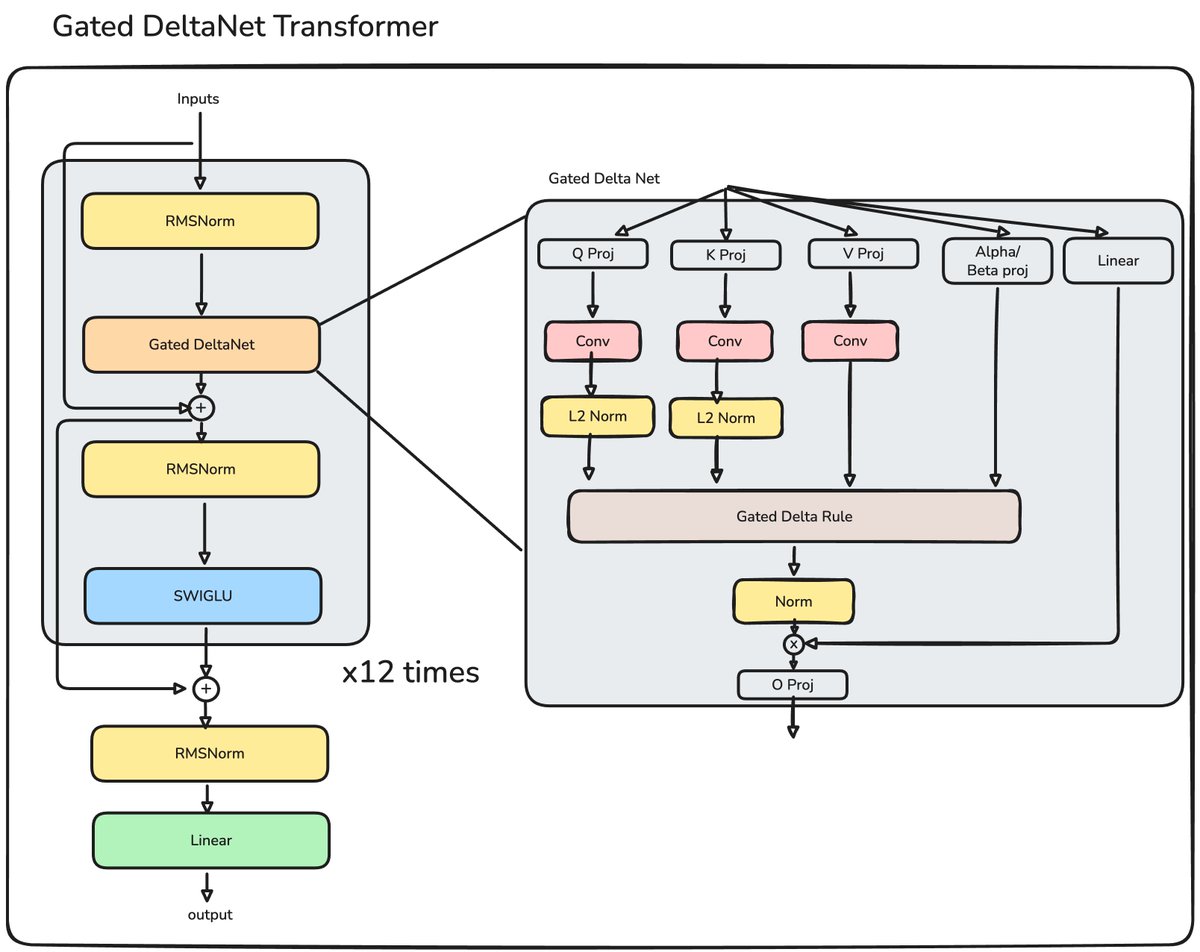
Remaining limitation: \alpha_t is typically a scalar per head. Identity, product, date, risk, sentiment, compliance may all decay together. The model cannot easily say: forget the stale date, keep identity and compliance.
13. Kimi Delta Attention: channel-level forgetting
Kimi Delta Attention (KDA) replaces scalar decay with a vector-valued diagonal gate \alpha_t \in [0,1]^{d_k}:
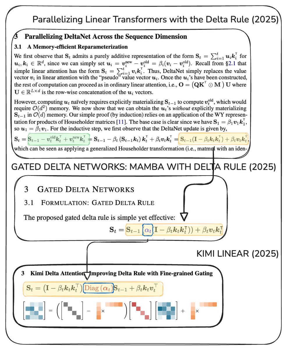
Conceptual decay vector:
→ preserve identity; mostly keep product; rapidly forget date; keep risk status. Learned channels are distributed features, not named fields—but the principle is multi-timescale memory inside one head.
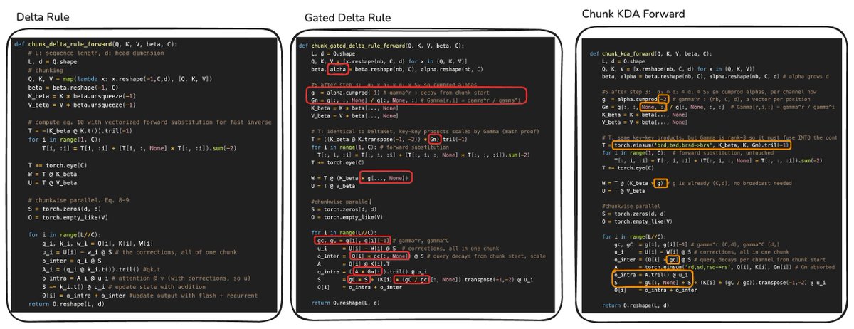
Why fine-grained decay is powerful
| Short-lived | Long-lived |
|---|---|
| Punctuation / local syntax | User objective |
| Temporary code expression | Entity identity / contract constraint |
| Local discourse glue | Session-level instruction |
14. KDA as a structured state-transition system
That is a specialised diagonal-plus-low-rank (DPLR) structure: efficient channel-wise decay + rank-one delta edit. Constraining the form enables chunkwise parallel GPU kernels (algorithm–hardware co-design) (Kimi Linear paper).
15. Chunkwise parallelism: recurrence that GPUs like
Recurrence S_1 \rightarrow S_2 \rightarrow \cdots \rightarrow S_n looks sequential. KDA (like DeltaNet) divides the sequence into chunks:
- intra-chunk — algebraically combine updates; pack rank-one transforms; parallel matmuls
- inter-chunk — pass final state as next chunk’s initial state
The important point is not only a clever recurrence—it is a recurrence that becomes hardware-efficient training kernels.
16. Why pure linear attention is still insufficient
The entire past must ultimately live in a fixed-size state.
Tasks that need exact access to many independent items (long random copy, unique IDs among thousands, multi-doc evidence, exact quotations) hit an information bottleneck. The Kimi report identifies long-context retrieval as a major limit of pure linear attention.
17. Kimi Linear: compressed memory + global retrieval
Kimi Linear interleaves:
- 3 × KDA layers
- 1 × full Multi-Head Latent Attention (MLA) layer
3 KDA : 1 MLA (reported strongest quality–throughput balance in their ablations)
| KDA layers | MLA layers |
|---|---|
| Efficient recurrent memory | Global token-to-token access |
| Selective decay + delta correction | Precise context retrieval |
| Lower KV-cache pressure | Relieves finite-state bottleneck |
Two memory systems:
- Compressed working memory (KDA) — update, correct, forget selectively
- Explicit episodic access (periodic full/MLA attention) — inspect original tokens when needed
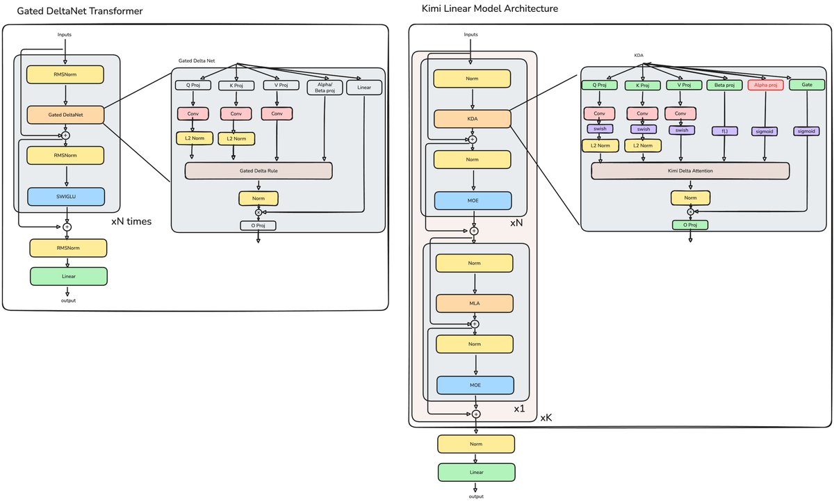
Reported matched experiments (author setup): reduced KV-cache use by up to ~75% and up to ~6× higher decoding throughput at 1M-token context for the evaluated configuration (arXiv:2510.26692).
18. The larger Kimi Linear model (reported config)
| Property | Reported |
|---|---|
| Total parameters | ~48B |
| Activated per token | ~3B |
| Context | up to 1M tokens |
| Token mixing | KDA + MLA hybrid |
| Channel mixing | sparse MoE |
19. How KDA improves long-context reasoning
KDA is not a standalone “reasoning algorithm.” Quality still depends on data, scale, optimisation, SFT/RL, tools. KDA improves the memory substrate:
- Reduced interference (delta correction)
- Multi-timescale memory (channel-wise decay)
- Efficient long trajectories (fixed state on most layers)
- Periodic global retrieval (MLA)
- Better resource allocation (expensive global attention only periodically)
Especially relevant for agentic loops: reason → tools → results → revise → act again.
20. Worked example: updating customer information
Conversation:
“My current broadband plan is Silver.”
“My customer number is 48192.”
“I have now upgraded to Platinum.”
“The old monthly fee was $45.”
“The new fee is $70.”
“Please compare my new plan with the old one.”
| Mechanism | Behaviour |
|---|---|
| Full attention | Directly retrieve Silver, Platinum, $45, $70, 48192 from KV archive (precise, cache-heavy) |
| Basic linear | plan→Silver then plan→Platinum may interfere |
| DeltaNet | Corrects plan association toward Platinum via prediction error |
| Gated DeltaNet | Can decay old topic state; scalar gate may blunt several features together |
| KDA | Different decay rates: forget active-plan Silver quickly; keep customer id, old fee for comparison, new plan/fee |
| Hybrid + MLA | Exact earlier text available when comparison needs literal retrieval |
21. Architectural comparison
| Property | Full softmax | Basic linear | DeltaNet | Gated DeltaNet | KDA |
|---|---|---|---|---|---|
| History | Explicit KV | Fixed matrix S | Fixed S | Fixed S | Fixed S |
| Main update | Pairwise attn | Additive outer product | Error-correcting delta | Delta + scalar decay | Delta + channel-wise decay |
| Forgetting | Truncate cache | None explicit | No broad forget | Head-wise adaptive | Channel-wise adaptive |
| Retrieval | Direct token↔token | From compressed state | Better associative | + lifespan control | Fine-grained management |
| Seq. cost | O(n^2) | O(n) | Linear recurrent | Linear recurrent | Linear recurrent |
| Decode mem. | KV grows with n | Fixed state | Fixed | Fixed | Fixed |
| Weakness | Cache/compute | Interference | Stale memory | Coarse forget | Still finite-state; complex kernels |
| Practice | Optimised FA/MLA | Often hybridised | Often hybridised | Often hybridised | Hybrid KDA + MLA |
22. Library analogy (memory-management interpretation)
| Stage | Analogy |
|---|---|
| GPT-2 full attention | Keep every document in an indexed archive |
| Linear attention | One continuously updated summary board |
| DeltaNet | Correct the summary before adding |
| Gated DeltaNet | Decide when to clear large sections |
| KDA | Control lifespan of individual “ink colours” / channels |
| Kimi Linear | Keep both a summary and periodic archive access |
23. Deeper evolution of Transformer architecture
- Passive storage → active memory control (write strength, correction, forget rates)
- Uniform timescales → learned timescales
- One architecture → hybrids (global, window, SSM/linear, MoE, external retrieval, tools)
- Mathematical elegance → hardware-aware design (chunkwise matmul-friendly forms)
- Short prompts → long-horizon agents (plans, tool traces, code, browsing, self-corrections)
24. What each generation really solved
| Generation | Solved | Did not solve / introduced |
|---|---|---|
| GPT-2 / full attn | Flexible global deps + general AR pretraining | Efficient ultra-long context |
| Linear attention | Quadratic cost / growing KV for those layers | Finite-state interference |
| DeltaNet | Uncontrolled additive writing | Indefinite survival of stale state |
| Gated DeltaNet | Adaptive erasure | Coarse scalar head-wise decay |
| KDA | Fine-grained multi-timescale decay | Pure linear capacity limit |
| Kimi Linear | Hybrid KDA + MLA coexistence | Not “end of history” |
| Kimi K3 | Scale + AttnRes + gated MLA + latent MoE | Still trails top proprietary models overall (per Moonshot’s own framing) |
25. Kimi K3: scaling the hybrid memory stack
Kimi K3’s language backbone follows the Kimi Linear pattern: 23 four-layer macrocycles, each with 3 KDA + 1 MLA, first FFN dense then latent MoE thereafter; context up to 1M tokens; native vision; open ~2.8T-class MoE (Kimi K3 blog).
Beyond “just bigger”:
- Blockwise Attention Residuals (AttnRes) every ~12 layers
- MLA query LoRA and output gating (Gated MLA)
- Latent-space MoE (e.g. 2 shared + 16-of-896 routed experts in public descriptions)
- SiTU activations
- KDA constant-state memory + periodic softmax/MLA retrieval
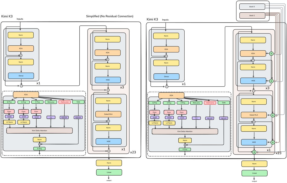
Gated MLA, latent MoE, SiTU
Gated MLA controls how much retrieved MLA content enters the residual stream via an input-dependent gate.
SiTU-style expert activation (conceptual):
d = x.shape[-1] // 2
gate = x[..., :d].to(torch.float32)
up = x[..., d:].to(torch.float32)
situ_a = self.beta * torch.tanh(gate / self.beta) * torch.sigmoid(gate)
if self.linear_beta is not None:
    up = self.linear_beta * torch.tanh(up / self.linear_beta)
return (situ_a * up).to(x.dtype)
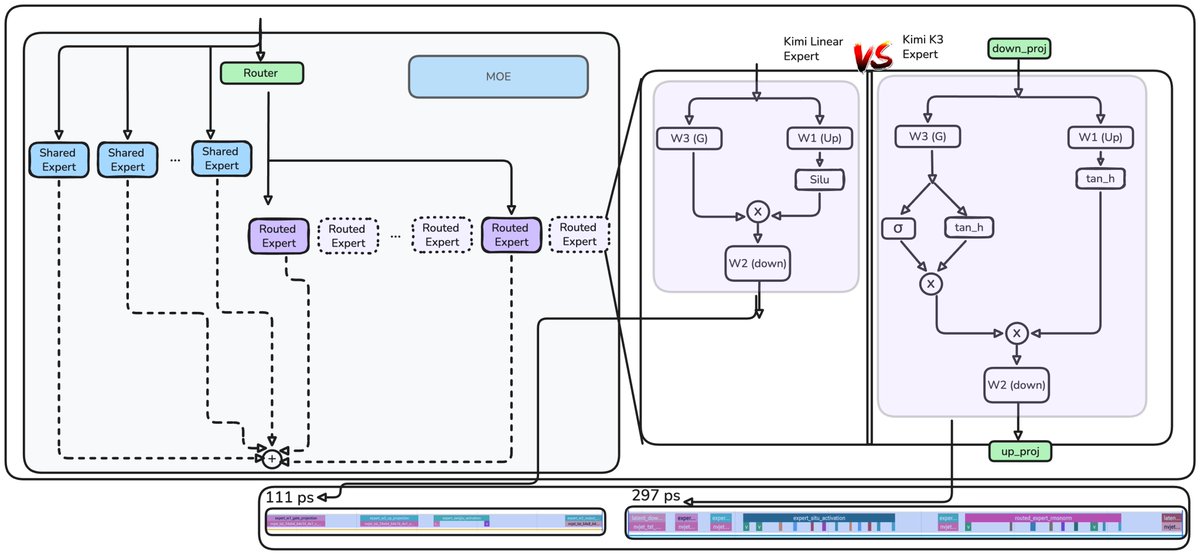
Without fused kernels, new activations can be much slower than SiLU paths; operating experts in a compressed latent space offsets cost by cutting FLOPs.
Attention Residuals (AttnRes)
Standard residuals give every preceding layer equal weight in the sum. Later layers must emit large deltas to move the stream; different layer types (KDA vs MLA vs MoE) may want different mixtures.
AttnRes instead forms a softmax-weighted combination of earlier residual-stream (or block) states using learned queries against normalised keys. Applied at block granularity (~every 12 layers) to keep cost manageable (~2% latency trade for reported training efficiency gains).
Conceptual block mixing:
V = torch.stack(blocks + [partial_block])  # [N+1, B, T, D]
K = norm(V)
logits = torch.einsum("d,nbtd->nbt", proj.weight.squeeze(), K)
h = torch.einsum("nbt,nbtd->btd", logits.softmax(0), V)
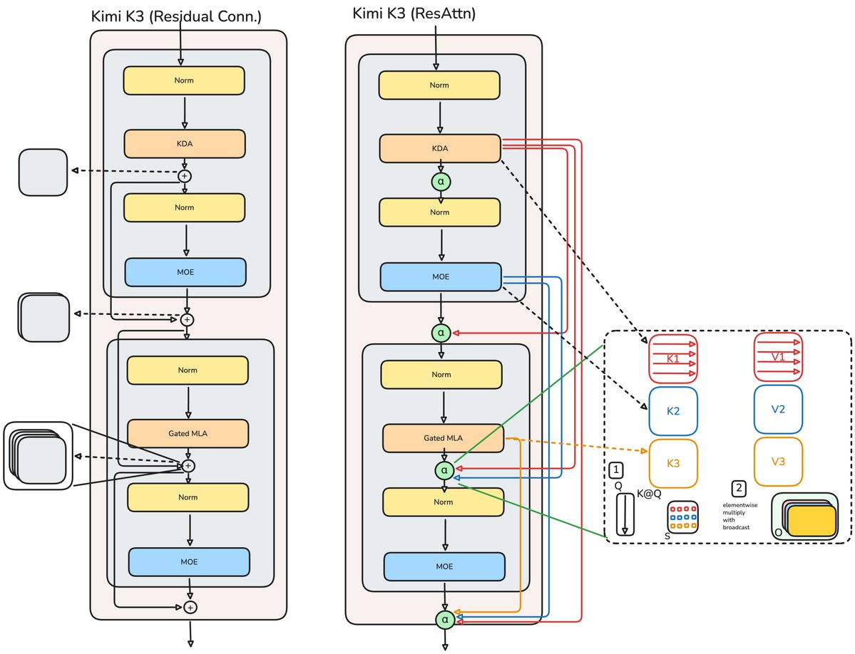
Interpretation:
- KDA — selective forgetting across time
- AttnRes — selective retrieval across depth
- MLA — selective retrieval across token context
Together: a fixed-capacity associative memory needs an eviction policy; learned selection (gating, routing, decay) plus occasional full attention is how modern stacks stay both efficient and precise.
26. Is KDA the final stage?
No. Follow-on work such as Gated DeltaNet-2 explores decoupling erase vs write more cleanly (arXiv:2605.22791). Likely directions: independent control of retention, erasure, writing, retrieval, consolidation, uncertainty, cross-layer communication, and external memory.
Conclusion
The advancement of Transformer architecture is not only a story of parameter counts—even when the ratio is 22,580× from GPT-2-scale to Kimi K3.
It is a progression in how systems represent and manage context:
Attention as retrieval
  → Attention as compressed memory
  → Attention as editable memory
  → Attention as selectively forgetful memory
  → Hybrid intelligent memory (time + depth + tokens + experts)
GPT-2-style Transformers treated context as an explicit token-level archive. Linear attention compressed it into a recurrent state. DeltaNet corrected associations; Gated DeltaNet forgot adaptively; KDA forgot per channel. Kimi Linear / Kimi K3 recognised that no fixed-size state replaces exact retrieval—so they keep periodic global MLA, then add sparse experts and (on K3) Attention Residuals.
Modern AI is evolving from a model that merely reads its context into a system that learns how to store, update, forget, and retrieve information according to the needs of an ongoing task.
Sources and further reading
- Original worklog (diagrams): 22580: From GPT2 to Kimi3, Explained — ali @waterloo_intern / status
- Attention Is All You Need
- GPT-2 report
- Transformers are RNNs: Linear Attention
- DeltaNet (parallel delta rule)
- Gated Delta Networks
- Kimi Linear: An Expressive, Efficient Attention Architecture
- Kimi K3 announcement
- Gated DeltaNet-2
Diagrams in this article are from the public X Article by @waterloo_intern; theoretical synthesis combines that worklog with the memory-management framing above and the cited papers.
Discussion
Comments
Share feedback or questions about this page. No account required.
Loading comments…